Cerebral cortex
A single neuron is a rather useless thing.
The three main axes of brain organization
Now for something completely different. Look at the image below. What do you see?
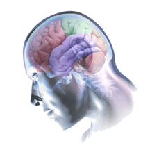
The skin and skull of this person have been made transparent to reveal the brain structures underneath. Not only that, but the brain itself has been tinted to highlight its major divisions.
Question
How many do you see?
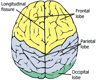
Longitudinal: The cerebral lobes
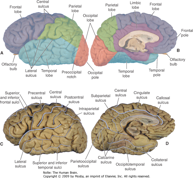
Well, behind the ear there is a purple mass of convolutions called the temporal lobe - which you can see better in Fig. 63. In front of it is a larger red mass called the frontal lobe; behind the temporal lobe is a smaller orange mass called the occipital lobe. Between the two along the top is a green mass called the parietal lobe. These four lobes make up what we usually think of as the brain, called the cerebrum. Beneath it and to its back is a brownish mass called the cerebellum, about which I will have very little to say in the course.
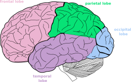
Fig. 63 The four lobes of the lateral surface of the left hemisphere. [2]
With the help of the landmarks of the face and ear, it is easy to see that the image presents the left side of the brain. But not so fast – the images that we deal with will not usually have these helpful guideposts. Consider the two below. They are also left sides, but how can you tell for sure?
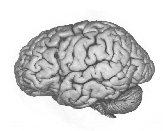
The obvious clue is the cerebellum, which is always at the back. More subtle is the direction of the temporal lobe. If you can discern its tip, it always points forward.
The next image is a crude approximation to how functions are arrayed across the lateral surface of the left hemisphere:
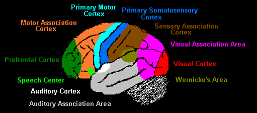
The occipital lobe mainly processes vision and the temporal lobe, audition. Down the front of the parietal lobe runs a thin strip of somatosensory cortex, which is the term for touch in medical science. So the rear of the cerebrum deals with the three main human senses: vision, audition and touch. Taste and smell are tucked underneath the cerebrum, out of sight so far. Between the primary sensory areas are zones of sensory combination called association areas. Across the way from somatosensory cortex at the rear of the frontal lobe is a strip of motor cortex, from whence movement is initiated. Moving forward, it is mediated by an association area to the most mysterious bit of all, the prefrontal cortex.
Lateral: The two hemispheres
The next image pivots our perspective from the left side to the top.
The two sides or hemispheres appear to be mirror images of each other, and at this coarse resolution we can think of them at such. But at a much finer level of resolution, that of networks of individual neurons, there are structural differences between the two hemisphere that permit them to specialize for different functions. Most language processing takes place in the left hemisphere, which is why I want you to be familiar with the brain or cerebrum viewed from its left side.
Up and down in the brain
The final axis of brain organization is the vertical one. The image below shows the structures which the cerebrum sits on and mostly covers:
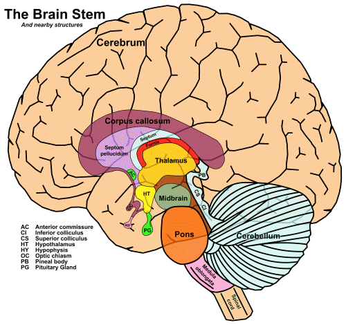
We will mainly be concerned with the cerebrum, though the thalamus will make an appearance every now and then.
How to name parts of the cerebrum that are smaller than a lobe
There are three conventions for naming smaller zones of the cerebrum.
Gyri and sulci
As is apparent in the images, the cerebrum is covered with folds called convolutions. A single fold has a high point, called a gyrus and a low point, called a sulcus, as in the diagram below:
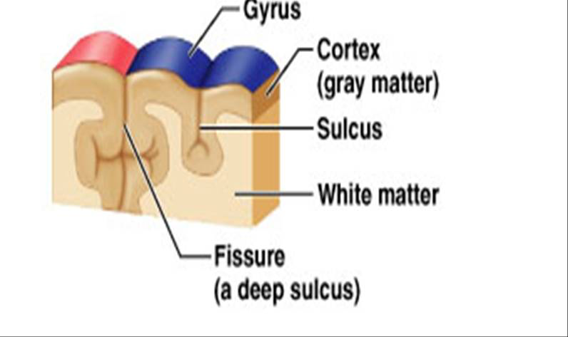
Fig. 65 Close-up of the cerebrum showing major landmarks. [4]
The organization and placement of the gyri and sulci does not change very much from person to person (we hope!), so there are standard names for them. We start with the gyri, the plural of gyrus:
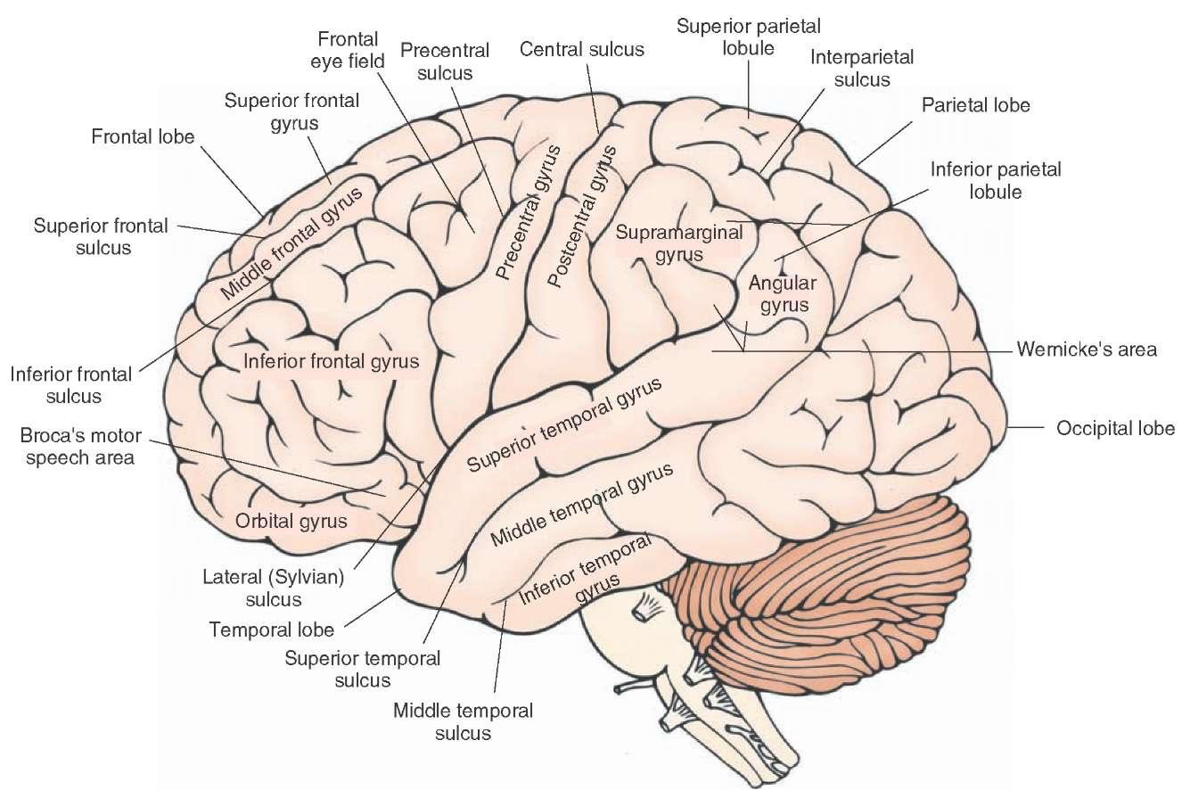
You should be able to recognize the superior temporal gyrus (STG), Wenicke’s area, the middle temporal gyrus (MTG), and the inferior frontal gyrus (IFG).
I should point out that so far, we have been looking at the lateral surface of the left hemisphere, but if you peeled back the left hemisphere above you would be looking at the medial surface of the right hemisphere:
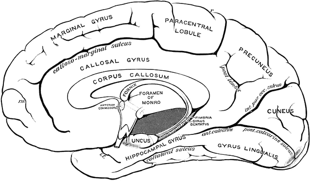
None of these areas play a direct role in language, so I will rarely refer to them – despite there being something called the gyrus lingualis!
Here are the sulci:
The lateral sulcus – AKA the Sylvian fissure – is the landmark around which the linguistic areas of the cortex are arrayed. Also important is the superior temporal sulcus (STS).
Speaking of acronyms …
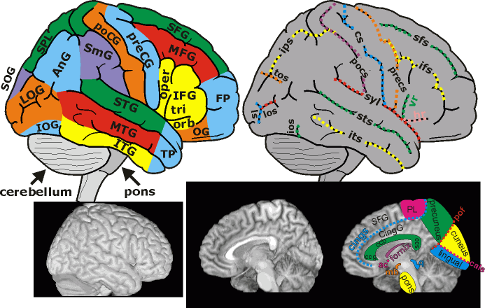
Fig. 69 Acronyms of major cortical landmarks.
Brodmann’s areas
In 1885 Franz Nissl wrote his doctoral dissertation on the constituents of neurons drawing on the microscopic examination of brain slices stained with a new technique that he had developed. Now known as the Nissl method or Nissl stain, it produces images such as this one:
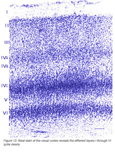
It is immediately apparent that cortex is divided into several layers, a property that you will learn about in Cerebral lamination.
A German anatomist named Korbinian Brodmann meticuously applied the Nissl method to all areas of the human cortex and discovered subtle variations in the layering which he complied into a map of the human cerebral cortex, published in 1909. His orignal illustration was in black and white with the areas that he identified distinguished by different markers. This version colorizes the markers to make the extent of each area pop out at you:
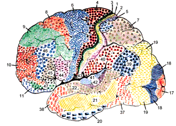
Fig. 71 Original cortical atlas by Brodmann, colorized lateral view of left hemisphere. [9]
Notice that Brodmann labelled each area with an integer. Look at them very carefully.
Question
Can you figure the way in which Brodmann sequenced the numbers?
Note
In this and the upcoming images, look for BA 41, 42, 22, 45 and 46.
Here is a version of his map colored by lobe:
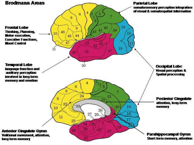
Fig. 72 Brodmann’s areas colored by lobe with an indication of general function. Lateral left hemisphere and medial right hemisphere. [10]
Here is a version also colored by lobe but labeled by gyrus and sulcus:
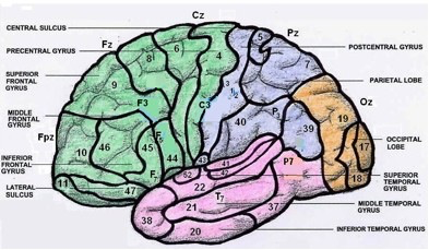
Fig. 73 Brodmann’s areas colored by lobe and labeled by gyrus and sulcus. Lateral left hemisphere. [11]
Finally here is a version colored by function:
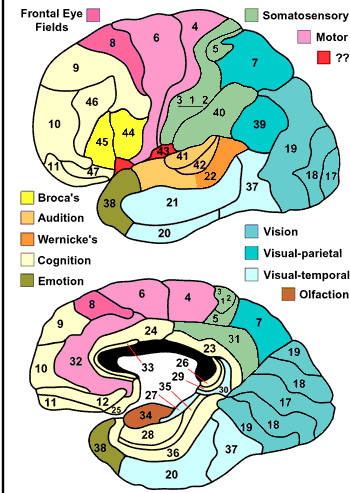
Fig. 74 Brodmann’s areas colored by function. Lateral left hemisphere and medial right hemisphere. [12]
 See the pdf at Cortical Functions for an overview of what every Brodmann area is thought to do.
Stereotaxic coordinate systems
Individual brains vary enough that it is helpful to ‘normalize’ an image of one to a standard template. After normalization, it is possible to report locations using three numbers or dimensions, called X, Y and Z. These dimensions refer to left-right (X), posterior-anterior (Y), and ventral-dorsal (Z). In Talairach coordinates, these numbers describe the distance from the ‘origin’ of Talairach space in the anterior commissure.
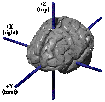
This permits great precision in the localization of an area of interest in the brain:
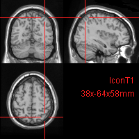
Fig. 76 A point located on the three planes of Talairach space.
Question
The image highlights the point 38x64x58. What would you call this spot in the other two naming conventions?
Despite the precision of Talairach coordinates, no one really refers to them in the discussion of cortical phenomena. The gyrus-sulcus and Brodmann systems are preferred, which is why I have dedicated so much time to them.
Connections and white matter
As you learned in the chapter on the Neuron, a spike chain is propagated to other neurons along a neuron’s axon. Axons bunch together into tracts that make up the white matter under the gray matter of the cell bodies.
Turning back to the left side – OK, is this really the left side? – this photograph of a brain sliced roughly front to back reveals that what you see on the surface does not extend very deep. Called grey matter, it consists mainly of neuronal cell bodies. These cell bodies are the main processors of the brain and their number increased dramatically in the evolution of reptiles to mammals. In this sense, they are ‘new’, and so the grey matter of the cerebrum is often known as neocortex, from the Latin words for “new” and “tree bark”.
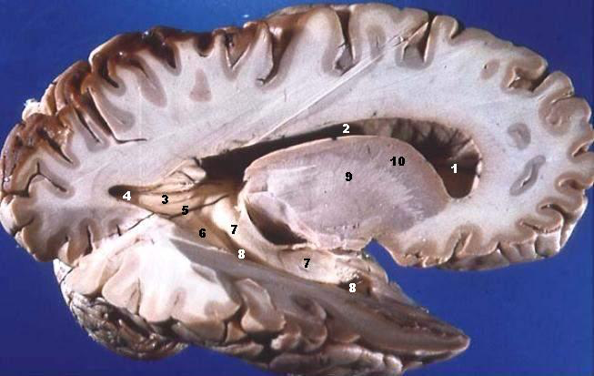
Fig. 77 Dissected brain showing the distinction between grey and white matter. [14]
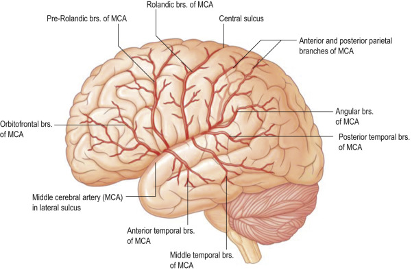
Blood flow
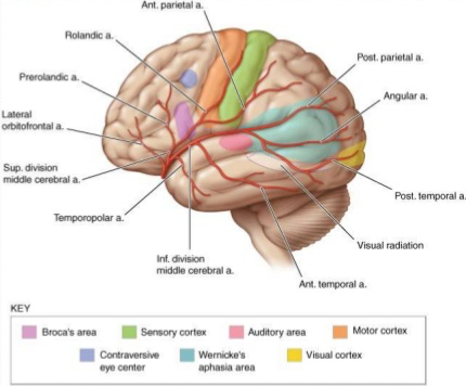
Fig. 78 The middle cerebral artery of the left hemisphere. [15]
Cytological architecture
Cerebral lamination
Columnar organization of neocortex suggests a certain layering of neocortex, and this is indeed the case. Mammalian neocortex is conventionally divided into six layers or laminae, according to where the soma and dendrites of pyramidal neurons bunch together. The traditional convention is to label each layer with a Roman numeral from I to VI, where layer I lies under the pia, the membrane just under the skull that protects the brain, and layer VI lies on top of the white matter, the bundles of fiber that connect individual areas of the cortex. Layering of neocortex, schematized by outputs of pyramidal cells gives a very schematic diagram of what this looks like. For instance, the soma of neurons whose output propagates to cortex nearby in the same hemisphere of the brain tend to bunch together in layer II, whereas the soma of neurons whose output propagates to the corresponding cortical area in the other hemisphere of the brain tend to bunch together in layer III. Recent usage prefers to conflate these two layers and further subdivide layer IV – and to use Arabic numbers for the Roman ones.
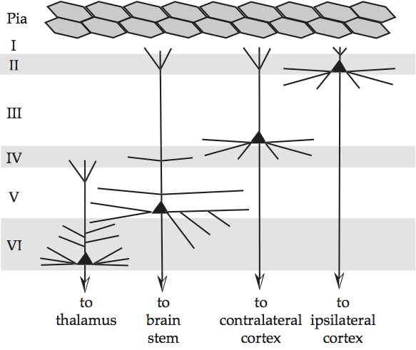
Fig. 79 Layering of neocortex, schematized by outputs of pyramidal cells
source: Howard Fig. 1.12. Comparable to Hendry, Hsiao and Brown, 1998, Fig. 23.7, Jones (1985), and Douglas and Martin, 1998, Fig. 12.8.
There is a fairly strict hierarchical pathway through these laminae, which follows the feedforward path of 4 → 2+3 → 5 → 6 and the feedback path of 5 → 2+3 and 6 → 4.
[MT18] proposes a two-layer, fast-slow system “… we use both fast and slow weights in parallel layers. The model’s slow weights learn deep representations of data. Its fast weights implement a Hebbian-learning-based associative memory [7, 10, 12], which binds class labels to representations in a single shot.”
Minicolumn
The smallest processing unit of a human brain is thought to be a two-dimensional array of anatomically identical minicolumns, each a group of a few hundred neurons whose somas occupy a cylinder approximately 25-50 mm in diameter, see Hendry et al., 1999, p. 666 or Kandel and Mason, 1995, p. 432 for an overview and Mountcastle (1997) for a more detailed review. Minicolumns are the functional units of sensory cortex, and also appear to be the functional units of associative cortex, see Mountcastle (1997).
They fulfill this role through a circuit design like that of Columnar organization of neocortex.
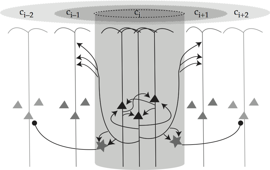
Fig. 80 Columnar organization of neocortex
source: Howard Fig. 2.6, comparable to Spitzer, 1999, Fig. 5.3.
Each minicolumn is composed of three pyramidal neurons and two smooth stellate interneurons, the latter of which are omitted from all but the central minicolumn of Columnar organization of neocortex for the sake of clarity. The diagram focuses on the central minicolumn, labeled i, showing how pyramids within it excite one another and the co-columnar stellate cells. Moreover, since a pyramidal cell’s basal dendrites radiate laterally from its soma for up to 300 mm, it can sample input from axons in minicolumns other than its own. In this way, the pyramidal cells in minicolumn i can also excite neurons in contiguous minicolumns, as depicted by the arrows from i to its two flankers i±1. The flankers are not excited enough to become active all by themselves, but they are excited enough to respond more readily to similar signals. Finally, the stellate interneurons are inhibitory, so their excitation inhibits the pyramidal cells at the further remove of minicolumns i±2. In this way, an excitatory ‘halo’ extends around the active minicolumn i that dissipates with increasing distance from i. This halo is represented directly at the top of Columnar organization of neocortex and also indirectly by the shading of the pyramidal somas: the darker the color, the more active the cell is.
Laterality
Summary
End notes
Last edited: Aug 18, 2025