The neuron
Introduction
The previous chapter concluded with hair cells having transduced a mechanical input into a biochemical output which excites the neurons of the cochlea nucleus to produce spike trains. In this chapter you will just skim the surface of how neurons produce spikes.
As Wikipedia says about the neuron, it is “… an electrically excitable cell that receives, processes, and transmits information through electrical and chemical signals.” Almost all of this book concentrates on the work-horse of the (neo)cortex, the (spiny) pyramidal cell, which comprises 75-80% of cortical cells, even though some of the pictures in this chapter illustrate a more general, multipolar neuron.
Structure of a pyramidal neuron
The pyramidal cells, as one might guess, have cell bodies shaped like pyramids. They mediate all long-range, and almost all short-range, excitatory influences in the cortex. Pyramidal cells can perform such mediation thanks to their extravagant design, which is depicted in an idealized form in Basic anatomy of a pyramidal cell.
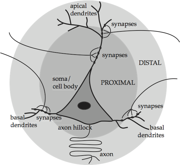
Fig. 53 Basic anatomy of a pyramidal cell
source: Howard Fig. 1.10
There are five main parts. The triangular shape in the lower middle contains the genetic and metabolic machinery of the cell and is known as the cell body or soma. The other four parts work together to channel the signals which enter the cell through synapses on its body and its dendrites, which are the web of fibers springing from the top and sides of the cell body. The prominent ascending dendritic shaft, called an apical dendrite, allows a pyramidal cell to form synapses in cortical layers above the layer in which its soma is located. Once in the cell, if the signals build up past a certain level, they initiate a electrical discharge at the axon hillock which travels down the long central channel or axon, and on to the next cells. Thus the fibers that synapse onto the cell in the picture come from the axons of other cells that are not shown. Given the importance of these terms for the upcoming discussion, they are summarized in Summary of the anatomy of an idealized pyramidal cell. Basic anatomy of a pyramidal cell also shades two zones around the soma, proximal for those neuron parts or neurites that are close to the soma, and distal for those neurites that are far from the soma.
Neurite |
Function |
|---|---|
Synapse |
Site of signal transmission from one neuron to another |
Dendrite |
Carries a signal towards the cell body |
Soma |
Body of the neural cell |
Axon hillock |
Juncture between soma and axon where signals are initiated |
Axon |
Carries a signal away from the cell body |
Neocortex also contains spiny stellate cells, and smooth or sparsely spinous interneurons. They are considerably less numerous and are usually not a focus of computational modeling. Spiny stellate cells are generally smaller than pyramids, and their cell bodies are vaguely star-shaped. They also sport spine-covered dendrites. The interneurons have more rounded cell bodies and little or no spines on their dendrites. Their axonal and dendritic arbors branch in a bewildering variety of patterns to which anatomists have given more or less descriptive appellations over the years. In a series of papers, Jennifer Lund and colleagues (Lund, 1987; Lund et al., 1988; Lund and Yoshioka, 1991; Lund and Wu, 1997) have described over 40 such subtypes in the macaque V1 alone. Such detail escapes the introductory goal of these pages, especially since it is not at all clear whether these anatomically distinct subtypes are physiologically distinguishable from one another.
How a neuron signals
The cell membrane
A cell is awash in a fluid that approximates seawater – more technically, a dilute aqueous solution of dissolved salts, mainly sodium chloride, NaCl, and potassium chloride, KCl. A cell’s internal environment consists of a similar aqueous solution, which is separated form the external solution by a two-level or bilayer of phospholipids known as the cell membrane.
The cell membrane regulates the exchange of molecules between the internal and external environments. Some molecules can diffuse right through the membrane, such as oxygen and carbon dioxide, because they dissolve in lipids. All others must have a specific means of transport. The cell membrane offers three different avenues. It is punctured here and there by small pores, as well as by larger, protein-lined channels, and it has embedded in it large globular proteins. The pores permit the diffusion of small molecules, such as water and urea, while the globular proteins attach to larger macromolecules such as sugars to pivot them across the membrane. A patch of cell membrane illustrates the lipid bilayer and a protein-lined channel, and also anticipates the chemical and electrical behavior of this structure.
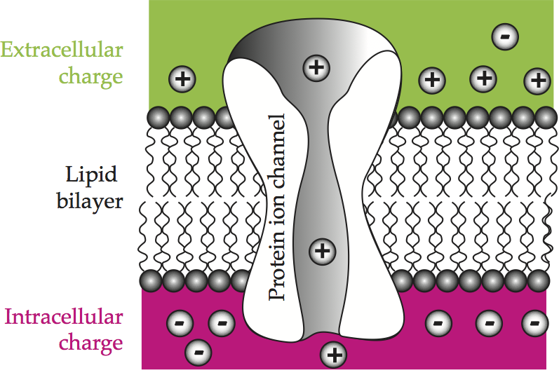
Fig. 54 A patch of cell membrane
Schematic representation of a patch of cell membrane showing an accumulation of charge across the insulating lipid bilayer and ion passage through protein channels. Comparable to Hille (1992). [Howard Fig. 2.1]
Ion channels and chemical and electrical gradients
What is of most interest to us are the protein-lined channels, for they permit the passage of the small ions that ultimately account for the electrical activity of neurons. There are two main kinds, sealable or gated channels, which can be open or closed, and passive or resting channels, which are always open. When a channel is open, any disparity between the ionic concentrations inside and outside the neuron will decrease.
The reason for this variety of selective ion channels is that a cell’s metabolism is constantly changing the concentration of ions and large molecules within it. If the concentration of these products were to become too large, osmotic pressure would force water into the cell, causing it to swell and burst. Thus for a cell to survive, it must have some means of regulating the concentration of the chemical species within it, and this is achieved mainly through the selective ion channels.
As was mentioned above, both the extra- and intracellular environments contain dissolved sodium and potassium chloride. These two salts disassociate into the ions Na+, K+, and Cl-. As a sample of how these ions can vary in concentration inside and outside a cell, the left side of Concentration of major ions and electrical potentials for squid giant axon, adapted from Keener and Sneyd, 1998, Table 2.1, relates their concentrations in the squid giant axon.
Ion |
Intracellular concentration |
Extracellular concentration |
Nernst potential |
Membrane potential |
|---|---|---|---|---|
Na+ |
50 mM |
437 mM |
+56 mV |
-65 mV |
K+ |
397 mM |
20 mM |
-77 mV |
– |
Cl- |
40 mM |
556 mM |
-68 mV |
– |
For all three ions, there is a marked asymmetry in concentration on either side of the axon membrane that produces a diffusion gradient from areas of high concentration to areas of low concentration. Under the influence of this gradient, the small potassium cation K+ readily diffuses through the passive channels and out of the cell, where it is much less abundant. In contrast, the low intracellular concentration of Na+ is maintained through a mechanism known as the sodium-potassium exchange pump, which uses energy to remove three atoms of Na+ against the sodium diffusion gradient of the extracellular fluid, while bringing in two atoms of K+ against the potassium diffusion gradient of the intracellular fluid.
The discussion of the movement of these ions under the influence of the various diffusion gradients ignores a crucial fact: their electrical charge. Given the differential concentration of ions between the interior and the exterior of a cell, an electrical charge accumulates on the interior surface of the cell membrane that exerts an electrical gradient across the cell membrane. Every potassium cation that leaves the cell makes its interior more negatively charged. The accumulation of negative charges starts attracting K+ back into the cell. Eventually, an equilibrium is reached at which the outflow and the inflow balance each other, and no more net change in accumulation takes place. The same holds for the other two ions, though the cell membrane has fewer channels through which they can pass, preventing them from playing a larger roll in the overall charge that builds up within the cell.
The difference in electrical potential across the membrane necessary to counterbalance the concentration gradient for a given ion is calculated by the Nernst equation, and the result is called the ion’s Nernst or equilibrium potential, \(E_ion\) or \(V_ion\). However, the Nernst equation is an idealization in that it assumes that only a single ionic species moves through an open channel. Given that there is a small probability that another ion of a similar size and charge will also pass through the same channel, it becomes necessary to use the Goldman or Goldman-Hodgkin-Katz equation, to find the actual potential in this mixed environment, called the reversal potential. If the probability of ‘contamination’ by different ions is small enough, the two equations produce the same results. The Nernst potentials for the squid giant axon are reproduced in the third column of Concentration of major ions and electrical potentials for squid giant axon.
The global charge that accumulates on the interior of the membrane from the mix of intracellular ions can be found by the Goldman-Hodgkin-Katz equation, and is called the membrane potential, \(V_m\). In a neuron, the membrane potential is also known as the resting state or resting potential of the neuron, Vrest, though it should be borne in mind that the membrane is not actually at rest; it is constantly expending energy to run the sodium-potassium pumps and so maintain the equilibrium between the influx and efflux of ions. In mammals, this expenditure accounts for half of the metabolic consumption of the brain, see Ames (1997). The membrane potential for the squid giant axon are reproduced in the fourth column of Concentration of major ions and electrical potentials for squid giant axon.
The action potential
If voltage is applied momentarily to the cell membrane of a ‘normal’, unexcitable cell, the membrane potential quickly returns to its resting state. However, in an excitable cell such as a neuron, the return to the initial state happens only if the voltage applied is below a certain value. If it is above this threshold value, the membrane potential shoots up to a maximum level, before falling precipitously back down to – and then below – its resting state. For instance, graphing the total membrane potential V over time reveals a single spike, which is modeled in Reaction of the cell membrane of an excitable cell to supra-threshold current input.
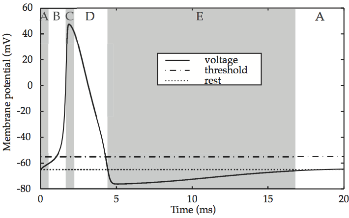
Fig. 55 Reaction of the cell membrane of an excitable cell to supra-threshold current input
source: Howard Fig. 2.4
In prose, the entire sequence consists of: (A) an initial resting state of the membrane potential of –65mV, (B) an upstroke (depolarization) up to (C) the excited state near 50 mV, (D) repolarization as the membrane potential returns to the resting state and then (E) a refractory period during which the potential overshoots the resting state and falls to –75mV, and (A) recovery to the resting state.
{Mussel and Schneider, 2021, #94782}
Action potentials are pulses that propagate along the membrane of excitable cells. The main types of excitable cells mentioned in classical textbooks are neurons and myocytes (e.g., Ref (Aidley and Ashley, 1998).). However, action potentials were detected in many other types of cells, and it is worth mentioning here in order to stress the generality of the phenomenon. A comprehensive list includes epithelial cells (Anderson, 1980), enteroendocrine cells (Strege et al., 2017), pancreas beta cells (Ribalet and Beigelman, 1980), glia cells (Káradóttir et al., 2008), fibroblasts (Lovisolo et al., 1988), osteoblasts (Pangalos et al., 2011), macrophages (McCann et al., 1983), taste buds (Roper, 1983), salivary glands (Kater et al., 1978), lung cancer cells (Blandino et al., 1995), oocytes (Schlichter, 1983), and many other types of cells in corals (Leys et al., 1999), plants (Fromm and Lautner, 2007), fungi (Slayman et al., 1976), and unicellular organisms (Wood, 1982). Thus, excitable cells were identified in organisms from all eukaryotic kingdoms. It is not clear if prokaryote cells are also excitable, although there are some positive hints (Kralj et al., 2011). The extent of excitability of intracellular organelles and vesicles is also not clear. However, excitability of the vacuole (a type of membrane-bound organelle) in Characean alga, is well known (Wayne, 1994).
The most common method to detect action potentials is by measuring the electric potential difference across the cell membrane. However, it has been demonstrated that additional non-electric aspects co-propagate with the electrical signal, including a nano-scale deformation of the cell surface, an adiabatic change of temperature, and changes in the optical properties of the cell (Tasaki, 1999). Some researchers have been arguing that these additional aspects should not be treated as an epiphenomenon, but rather that a major shift from the classical electrical paradigm of action potentials should be considered (Tasaki, 1982; Sutherland, 1905; Doerner, 1969, 1971; Kaufmann, 1989; Heimburg, 2008). The theory of sound in lipid membranes near phase transition is a promising framework that unifies much of the observed phenomenology.
Computation and the cell membrane
Keyes (1985) raises the question of what makes a good computational device, and answers with three desiderata. A “good” computational system is one that survives in the real world, for which it (i) must operate at high speeds, in order to anticipate and react to a fast-changing environment, (ii) must have a rich repertoire of computational primitives, in order to have a wide range of responses, and (iii) must interface with the physical world, in order to represent sensory input accurately and decide on appropriate motor output.
As Koch, 1999, p. 5, adds, the membrane potential of an excitable cell such as a neuron is “the one physical variable that fulfills these three requirements”. It can change its state quickly and over neurologically large distances; it results from the confluence of a vast number of nonlinear sub-states, the various ionic channels; and it is the common currency of the nervous system: visual, tactile, auditory, and olfactory stimuli are transduced into membrane potentials, and action potentials in turn stimulate the release of neurotransmitters or the contraction of muscles.
Electrical and hydraulic models of the cell membrane
The reader may have been surprised to see references to the squid giant axon in the preceding paragraphs – for, after all, the goal of all this neurophysiology is to understand that most human of abilities, language, and squid are not known for their linguistic proficiency. The reason for an unavoidable mention of cephalopods in an introduction to human neuroscience lies in the fact that the first measurements and models of the membrane signaling event were made on squid giant axons in the 1940’s and early 1950’s. Given the technique of inserting a glass micropipette electrode into the neurite to be studied, the giant axon of the North Atlantic squid Loligo pealei was a convenient target, because it is several centimeters long and one millimeter in diameter.
The size of microelectrodes has for decades limited the neurites whose electrical behavior can be studied to the axon and soma, and they continue to be the best known, and simplest, cases. For this reason, our initial models ignore dendrites and concentrate on the widest part of the neuron.
The earliest insight into the electrical behavior of a neuronal cell membrane is that it can be modeled by three electrical components, a capacitor, a battery, and a resistor. The insulating lipid bilayer acts like a capacitor in that a charge tends to build up on the inside wall of the cell membrane that is opposite in polarity to the charge outside the cell. The equilibrium potential of the cell acts like a battery that supplies current if some load on the circuit takes it out of equilibrium. The flow of ions through a protein channel acts like a resistor in the sense that the narrow protein channel restricts the flow of ions greatly. The standard circuit diagram for a capacitor and a resistor acting in parallel is given in Models of the cell membrane, which labels each component with the corresponding mathematical expression.
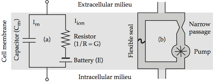
Fig. 56 Models of the cell membrane
(a) Equivalent electrical circuit. The left branch represents the displacement current Im, and the right branch represents the conduction current Iion; (b) analogous hydraulic circuit. source: Howard Fig. 2.2.
Since it is often difficult to grasp exactly what is happening in an electrical circuit without some formal training, Models of the cell membrane sketches a hydraulic analog to the direct current diagram which the reader may find more intuitively understandable. The flexible seal on the left branch bulges in response to current flow, thereby dividing its pipe into a half in which the fluid is compressed – building up positive pressure – and a half in which the fluid is rarefied – building up negative pressure. This is the hydraulic analog of a capacitor. The hydraulic pump corresponds to the electric battery as a source of current. The constriction in the pipe imposes a drag on current flow that reproduces a resistor’s impedance. Note that neither circuit has a direction of current flow imposed on it, since direction varies according to the ion.
The four-equation, Hodgkin-Huxley computational model
Hodgkin and Huxley (1952) devised one major equation and three supporting equations to model the signaling event in squid giant axons known as the action potential. This mathematical model describes the initiation and propagation of action potentials so well that, not only has it not been replaced in the intervening four decades, but rather has become the standard used for simulations of the squid giant axon, as well as the usual form in which equations for other cell membranes are cast – not to mention winning a Nobel prize for Hodgkin and Huxley in 1962.
The insight of Hodgkin and Huxley is that the Na+ and K+ conductance currents cross the membrane in separate but parallel pathways that are controlled by voltage, along with the passive diffusion of K+ that maintains the resting potential. Hodgkin-Huxley electrical circuit augments the electric circuit of Models of the cell membrane to reflect the contribution of each ionic term.
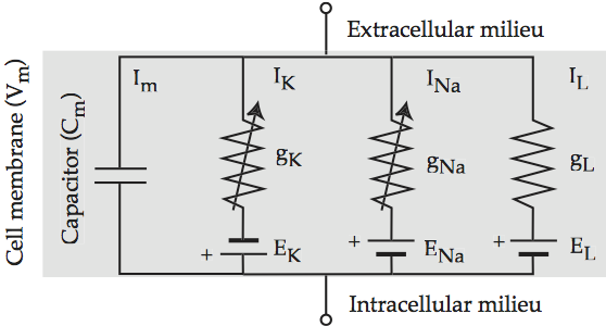
Fig. 57 Hodgkin-Huxley electrical circuit
Equivalent electrical circuit for the cell membrane that includes the three Hodgkin-Huxley ionic conductances. The arrows across the potassium and sodium resistors indicate that they are active, i.e. triggered by voltage. The leak resistor is passive. Source: Howard Fig 2.3
For completeness, the the full form of the Hodgkin-Huxley equation is:
Cm(dVm/dt) = –n4ḡK(Vm – EK) – m3hḡNa(Vm – ENa) – g ̄L(Vm – EL) + Iapp
When this system is perturbed from its equilibrium by the application of an external current, Iapp, the result is an action potential like the one of Reaction of the cell membrane of an excitable cell to supra-threshold current input, which in fact was calculated from this equation.
One of the most fascinating properties of the Hodgkin-Huxley model appears when an above-threshold stimulus is applied to it without interruption. The result is depicted in Hodgkin-Huxley spike train, What the graph shows is that, after some initial settling-in, the action potential repeats itself periodically and with no variation. This sequence of repeated firings of a neuron is known as a spike train. The fact that the Hodgkin-Huxley model produces spike trains is considered to constitute another confirmation of its empirical validity, given that trains such as those of Hodgkin-Huxley spike train have been observed repeatedly in living neural tissue.
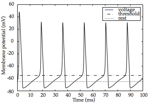
Fig. 58 Hodgkin-Huxley spike train
source: Howard Fig. 2.6
Dendrites
Todo
I am not sure how deeply more to go into neural microstructure.
Summary
References
Powerpoint and podcast
Endnotes
The next topic
Come to class having read Subcortical audition and answered the questions.
Last edited Aug 18, 2025